Filter a Pivot Table

The Spreadsheet provides numerous ways to apply filtering to the PivotTable fields to display only data that meets specific criteria. Select the task you wish to perform.

• Use a Report Filter
• Filter Row or Column Items
• Use a Label Filter
• Use a Date Filter
• Use a Value Filter
• Use Multiple Filters per Field
• Remove a Filter

Use a Report Filter

A report filter allows you to filter the entire PivotTable report to show data for specific items. To use a report filter, follow the steps below.

1. Click the arrow in the report filter field.

   

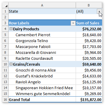
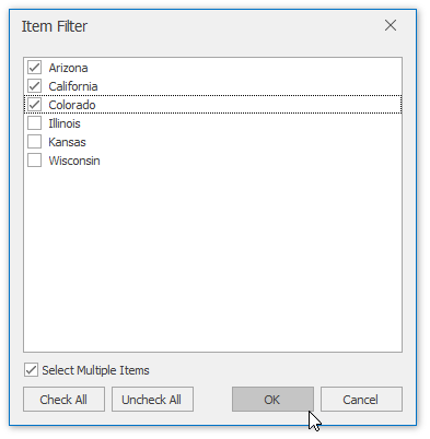
2. In the invoked dialog, click the Uncheck All button to deselect the values. Then, select the check box for the item you wish to display. To select multiple items, select the Select Multiple Items check box at the pane bottom. Click OK to apply changes.

   

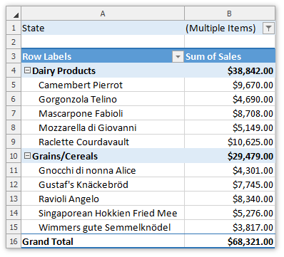
3. The resulting report is shown in the image below. The Filter button appears in the report filter field to indicate that the filter is applied.

   

Filter Row or Column Items

1. Click the arrow in the Row Labels or Column Labels cell. If there are multiple fields in the area, select the row or column field you wish to filter.

2. In the drop-down menu, select Item Filter...

   

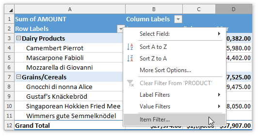
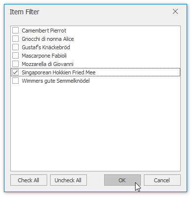
3. In the invoked dialog, click the Uncheck All button to deselect the values. Then, select the item(s) you wish to display and click OK.

   

4. The resulting report is shown in the image below. The Filter button appears in the row or column label to indicate that the filter is applied.

   

Use a Label Filter

1. Click the arrow in the Row Labels or Column Labels cell. If there are multiple fields in the area, select the row or column field you wish to filter.

2. Point to the Label Filters item and select one of the built-in comparison operators.

   

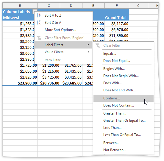
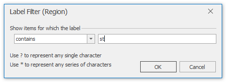
3. In the invoked dialog, specify the filter criteria and click OK.

   

4. The resulting report is shown in the image below. The Filter button appears in the row or column label to indicate that the filter is applied.

   

Use a Date Filter

1. Click the arrow in the header of the row or column field containing dates.

2. Point to the Date Filters item and select one of the built-in dynamic filter types to display dates that fall within a specified time period (next, this or last week, month, year, etc.) or select the Before, After, Equals or Between item to find dates that are before, after or equal to the specified date, or between two dates.

   

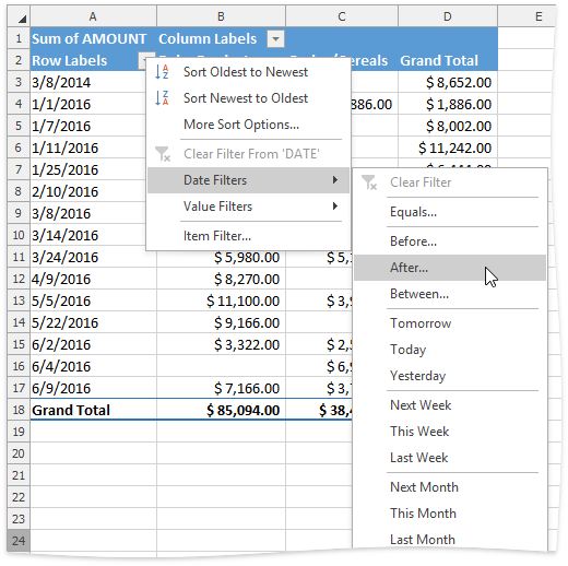
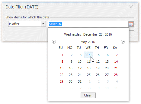
3. In the invoked Date Filter dialog, specify the date(s) to filter by and click OK.

   

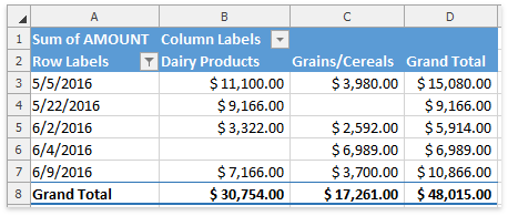
4. The resulting report is shown in the image below. The Filter button appears in the row or column label to indicate that the filter is applied.

   

Use a Value Filter

A value filter allows you to filter items in a row or column field based on summary values. To use a value filter, follow the steps below.

1. Click the arrow in the Row Labels or Column Labels cell. If there are multiple fields in the area, select the row or column field to which a filter should be applied.

2. Point to the Value Filters item and select one of the built-in comparison operators.

   

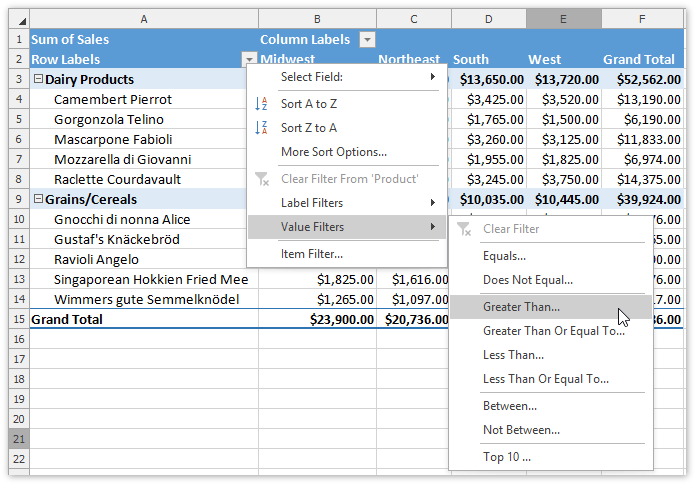
3. In the invoked dialog, specify the filter criteria and click OK. Note that the filtering will be applied to the filtered field's Grand Total values.

   

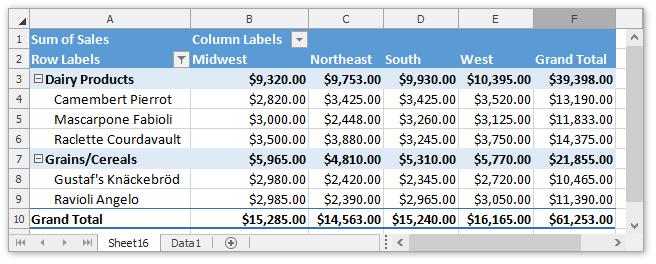
4. The resulting report is shown in the image below. The Filter button appears in the row or column label to indicate that the filter is applied.

   

Use Multiple Filters per Field

To enable the capability to apply multiple filters to a single row or column field, do the following.

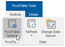
• On the PivotTable Tools | Analyze tab, in the PivotTable group, click the PivotTable Options button.

  

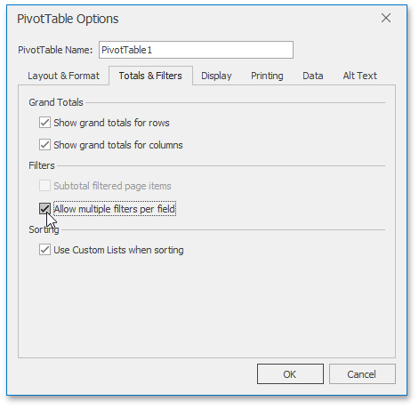
• In the invoked PivotTable Options dialog, switch to the Totals & Filters tab and check the Allow multiple filters per field box.

  

Remove a Filter

To remove a filter, do the following.

• To remove a filter from a specific field, click the Filter button and select the Clear Filter From 'Field Name' item in the drop-down menu.

  

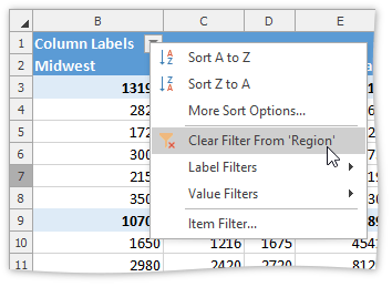
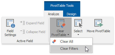
• To clear all filters applied to the PivotTable fields at once, on the PivotTable Tools | Analyze tab, in the Actions group, click Clear PivotTable | Clear Filters.