Freeze Columns and Rows

To keep specific columns and rows of the worksheet visible while scrolling through the rest of the worksheet, lock them in place using the Freeze Panes options of the Spreadsheet.

To freeze specific row(s) or column(s), follow the instructions below.

1. Depending on what you wish to freeze, do one of the following.

   • To lock a row(s), select the row below the row(s) you wish to freeze.
   • To lock a column(s), select the column to the right of the column(s) you wish to freeze.
   • To lock a row(s) and column(s) simultaneously, click the cell below the row(s) and to the right of the column(s) you wish to freeze.

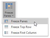
2. In the Window group within the View tab, click the Freeze Panes button's drop-down.

   

   Select one of the following.

   • Freeze Panes - lock multiple columns and/or multiple rows simultaneously.
   • Freeze Top Row - lock the first row only.
   • Freeze First Column - lock the left column only.

   A black border appears beneath the frozen row(s) and to the right of the frozen column(s).

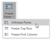
3. To unfreeze a row(s) or column(s), click the Unfreeze Panes item from the Freeze Panes button's drop-down list. This unlocks all frozen rows and columns in the worksheet.